Demo for how to calibrate PSF for estimating vessels diameters with super-localization#
import matplotlib.pyplot as plt
import numpy as np

from sl2pm import track_vessel
from sl2pm.models import L_wall_plasma, L_plasma_no_glx, L_wall
from sl2pm import misc
Protocol A (both plasma and wall fluorescence)#
Load wall- and plasma kymograms and average line-scans over time
kymo_wall = np.load('wall.npy')
kymo_plasma = np.load('plasma.npy')

N_AVER, nx = kymo_wall.shape
x = np.arange(nx)

data_wall = np.mean(kymo_wall, axis=0)
data_plasma = np.mean(kymo_plasma, axis=0)
Enter PMT parameters (known from the calibration)
ALPHA = 0.452
SIGMA = 6.0
GAIN = 3/ALPHA
Make an initial parameter guess
p0_A = track_vessel.ols_wall_plasma(data_wall/GAIN,
                                    data_plasma/GAIN,
                                    sigma_blur=1.5)
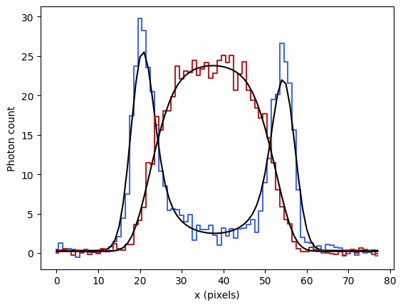
Plot data (staircase curves; blue – wall fluorescence, red – plasma fluorescence) and its expected value (black), evaluated with the initial parameter guess
plt.step(x, data_wall/GAIN, where='mid', c='royalblue')
plt.plot(x, L_wall_plasma(x, *p0_A)[0], c='k')

plt.step(x, data_plasma/GAIN, where='mid', c='firebrick')
plt.plot(x, L_wall_plasma(x, *p0_A)[1], c='k')

plt.xlabel('x (pixels)')
plt.ylabel('Photon count')
Text(0, 0.5, 'Photon count')
Fit the model
opt_res_A = track_vessel.mle(x,
                             np.array([data_wall, data_plasma]),
                             L_wall_plasma,
                             p0_A,
                             N_AVER,
                             ALPHA,
                             SIGMA,
                             minimize_options=dict(gtol=1e-3))
opt_res_A
  message: Optimization terminated successfully.
  success: True
   status: 0
      fun: 552.8399191026784
        x: [ 3.751e+01  2.099e+00  8.536e+00  1.188e+01  1.778e+01
             6.531e+00 -8.464e-02  2.077e+02  2.841e+01 -6.949e-01
             3.378e-01  2.293e-01]
      nit: 26
      jac: [-2.289e-05  1.831e-04  7.629e-06  7.629e-06 -7.629e-06
            -2.289e-05  2.289e-04  7.629e-06 -7.629e-06  7.629e-06
             3.815e-05  3.052e-05]
 hess_inv: [[ 6.007e-04  8.095e-05 ... -1.116e-05 -1.714e-05]
            [ 8.095e-05  1.834e-03 ... -4.374e-04 -1.701e-04]
            ...
            [-1.116e-05 -4.374e-04 ...  2.788e-03  4.485e-05]
            [-1.714e-05 -1.701e-04 ...  4.485e-05  2.294e-03]]
     nfev: 442
     njev: 34
Plot data (staircase curves; blue – wall fluorescence, red – plasma fluorescence) and its fitted expected value (black)
plt.step(x, data_wall/GAIN, where='mid', c='royalblue')
plt.plot(x, L_wall_plasma(x, *opt_res_A.x)[0], c='k')

plt.step(x, data_plasma/GAIN, where='mid', c='firebrick')
plt.plot(x, L_wall_plasma(x, *opt_res_A.x)[1], c='k')

plt.xlabel('x (pixels)')
plt.ylabel('Photon count')
Text(0, 0.5, 'Photon count')

List fitted parameters and their error bars
misc.fitted_params(opt_res_A, ['xc', 's_xy', 'l', 'R_lum', 'R_wall', 's_gcx', 'a1', 'Iw', 'Ip', 'b_plasma', 'b_tissue_wall', 'b_tissue_plasma'])
{'xc': (37.514531653402486, 0.02450966083760706),
 's_xy': (2.099006076364929, 0.0428280052806139),
 'l': (8.536404089959527, 1.1722363949232186),
 'R_lum': (11.87814031483626, 0.6952352469157619),
 'R_wall': (17.782737291476547, 0.07071767887009002),
 's_gcx': (6.530637072499391, 1.2606438821370647),
 'a1': (-0.08463889078707737, 0.008544453748425003),
 'Iw': (207.69979308370358, 13.314552526703766),
 'Ip': (28.41487072778165, 1.3117533870270208),
 'b_plasma': (-0.6948531659485018, 0.8490414048241006),
 'b_tissue_wall': (0.33780382098758993, 0.05279788934639521),
 'b_tissue_plasma': (0.2293084113470751, 0.04789879679981292)}
Protocol B (only plasma fluorescence)#
Load plasma kymogram and average line-scans over time
kymo_plasma = np.load('plasma.npy')

N_AVER, nx = kymo_plasma.shape
x = np.arange(nx)

data_plasma = np.mean(kymo_plasma, axis=0)
Enter PMT parameters (known from the calibration)
ALPHA = 0.452
SIGMA = 6.0
GAIN = 3/ALPHA
Make an initial parameter guess
p0_B = track_vessel.ols_plasma(data_plasma/GAIN, sigma_blur=1.5)
Plot data (red staircase curve – plasma fluorescence) and its expected value (black), evaluated with the initial parameter guess
plt.step(x, data_plasma/GAIN, where='mid', c='firebrick')
plt.plot(x, L_plasma_no_glx(x, *p0_B), c='k')

plt.xlabel('x (pixels)')
plt.ylabel('Photon count')
Text(0, 0.5, 'Photon count')

Fit the model
opt_res_B = track_vessel.mle(x,
                             data_plasma,
                             L_plasma_no_glx,
                             p0_B,
                             N_AVER,
                             ALPHA,
                             SIGMA,
                             minimize_options=dict(gtol=1e-3))
opt_res_B
  message: Optimization terminated successfully.
  success: True
   status: 0
      fun: 242.47981785380168
        x: [ 3.736e+01  2.578e+00  2.173e+01  1.662e+01  4.507e+01
             2.245e-01]
      nit: 17
      jac: [-4.578e-05  3.662e-04  5.531e-04 -7.515e-04 -3.700e-04
            -7.629e-06]
 hess_inv: [[ 3.132e-03 -4.821e-04 ...  4.547e-02  3.207e-05]
            [-4.821e-04  3.688e-02 ... -2.332e+00 -2.755e-03]
            ...
            [ 4.547e-02 -2.332e+00 ...  2.279e+02  1.037e-01]
            [ 3.207e-05 -2.755e-03 ...  1.037e-01  2.571e-03]]
     nfev: 154
     njev: 22
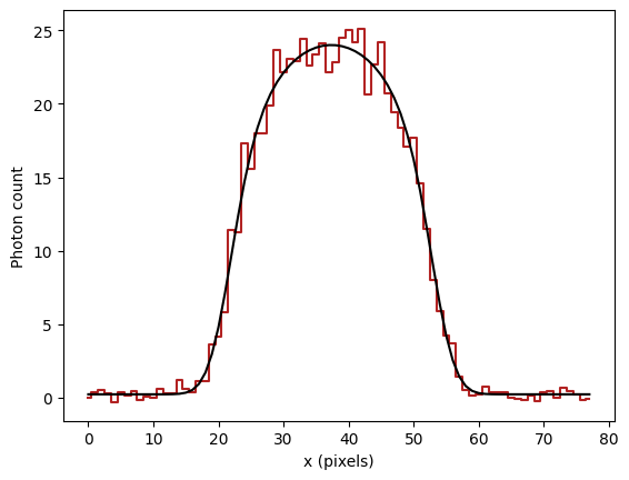
Plot data (red staircase curves – plasma fluorescence) and its fitted expected value (black)
plt.step(x, data_plasma/GAIN, where='mid', c='firebrick')
plt.plot(x, L_plasma_no_glx(x, *opt_res_B.x), c='k')

plt.xlabel('x (pixels)')
plt.ylabel('Photon count')
Text(0, 0.5, 'Photon count')
List fitted parameters and their error bars
misc.fitted_params(opt_res_B, ['xc', 's_xy', 'l', 'R_lum', 'I', 'b'])
{'xc': (37.357783286452765, 0.05596201173626481),
 's_xy': (2.5781221248626913, 0.19204302201772772),
 'l': (21.72527155350243, 11.12412896218862),
 'R_lum': (16.621259923594035, 0.2984907728269911),
 'I': (45.073374306794946, 15.096919840285185),
 'b': (0.2244572570512873, 0.05070972819669927)}
Protocol C (only wall fluorescence)#
Load wall kymogram and average line-scans over time
kymo_wall = np.load('wall.npy')

N_AVER, nx = kymo_wall.shape
x = np.arange(nx)

data_wall = np.mean(kymo_wall, axis=0)
Enter PMT parameters (known from the calibration)
ALPHA = 0.452
SIGMA = 6.0
GAIN = 3/ALPHA
Make an initial parameter guess
p0_C = track_vessel.ols_wall(data_wall/GAIN, sigma_blur=1.5)
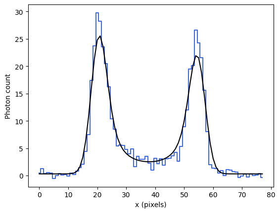
Plot data (blue staircase curves – wall fluorescence) and its expected value (black), evaluated with the initial parameter guess
plt.step(x, data_wall/GAIN, where='mid', c='royalblue')
plt.plot(x, L_wall(x, *p0_C), c='k')

plt.xlabel('x (pixels)')
plt.ylabel('Photon count')
Text(0, 0.5, 'Photon count')
Fit the model
opt_res_C = track_vessel.mle(x,
                             data_wall,
                             L_wall,
                             p0_C,
                             N_AVER,
                             ALPHA,
                             SIGMA,
                             minimize_options=dict(gtol=1e-3))
opt_res_C
  message: Optimization terminated successfully.
  success: True
   status: 0
      fun: 302.608023794074
        x: [ 3.755e+01  2.109e+00  8.115e+00  1.776e+01 -8.535e-02
             2.029e+02 -3.864e-01  3.362e-01]
      nit: 20
      jac: [ 0.000e+00 -1.526e-05  3.815e-06  1.526e-05 -6.104e-05
             0.000e+00 -1.526e-05  0.000e+00]
 hess_inv: [[ 7.384e-04  1.284e-04 ...  2.196e-03 -1.541e-05]
            [ 1.284e-04  1.834e-03 ...  2.251e-02 -4.536e-04]
            ...
            [ 2.196e-03  2.251e-02 ...  5.896e-01 -3.602e-03]
            [-1.541e-05 -4.536e-04 ... -3.602e-03  2.778e-03]]
     nfev: 243
     njev: 27
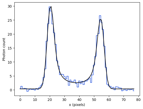
Plot data (blue staircase curves – wall fluorescence) and its fitted expected value (black)
plt.step(x, data_wall/GAIN, where='mid', c='royalblue')
plt.plot(x, L_wall(x, *opt_res_C.x), c='k')

plt.xlabel('x (pixels)')
plt.ylabel('Photon count')
Text(0, 0.5, 'Photon count')
List fitted parameters and their error bars
misc.fitted_params(opt_res_C, ['xc', 's_xy', 'l', 'R_wall', 'a1', 'I', 'b_plasma', 'b_tissue'])
{'xc': (37.55043704411089, 0.027172690949725672),
 's_xy': (2.108698966918546, 0.042826311232183015),
 'l': (8.114816413053992, 1.052837167955533),
 'R_wall': (17.76395751899086, 0.06915482348213965),
 'a1': (-0.0853471332327959, 0.008856287591524547),
 'I': (202.92446646762752, 11.779413529370489),
 'b_plasma': (-0.3863676128638186, 0.7678566563123971),
 'b_tissue': (0.3362464913776081, 0.05271136987249036)}