Demo for how to track a capillary (estimate radius and center position) with fluorescently-labeled plasma#
import matplotlib.pyplot as plt
import numpy as np

from sl2pm import track_vessel
from sl2pm.models import L_plasma_no_glx
from sl2pm import misc
Calibrating the microscope’s PSF#
Load kynogram
kymogram = np.load('plasma_kymogram_long.npy')
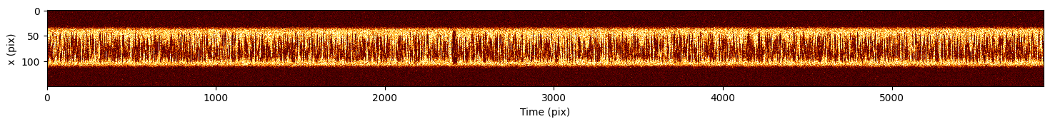
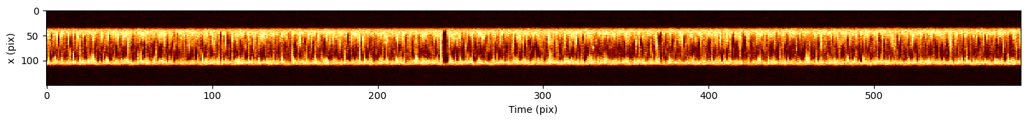
Plot the kymogram and find a segment without RBCs
fig, ax = plt.subplots(figsize=(18, 3))

ax.imshow(kymogram.T,
           cmap='afmhot',
           vmin=kymogram.min(),
           vmax=0.2*kymogram.max(), # manually selected maximum intensity for better visualization
           aspect=3,
          interpolation='none'
         )

ax.set_xlabel('Time (pix)')
ax.set_ylabel('x (pix)')
Text(0, 0.5, 'x (pix)')
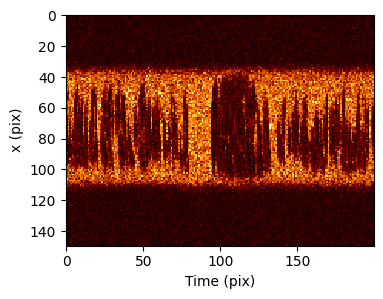
Roughly zoom-in into a potential RBC-free segment
kymogram_no_rbc0 = kymogram[2300: 2500]

fig, ax = plt.subplots(figsize=(18, 3))

ax.imshow(kymogram_no_rbc0.T,
           cmap='afmhot',
           vmin=kymogram_no_rbc0.min(),
           vmax=kymogram_no_rbc0.max(),
           aspect=1,
          interpolation='none'
         )

ax.set_xlabel('Time (pix)')
ax.set_ylabel('x (pix)')
Text(0, 0.5, 'x (pix)')
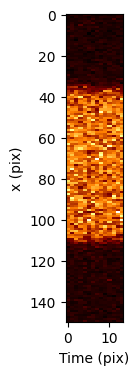
Select the RBC-free segment
kymogram_no_rbc = kymogram_no_rbc0[80: 94] # Vary the indexes to make sure you are not including RBC shadows into the RBC-free kymogram

fig, ax = plt.subplots(figsize=(6, 4))

ax.imshow(kymogram_no_rbc.T,
           cmap='afmhot',
           vmin=kymogram_no_rbc.min(),
           vmax=kymogram_no_rbc.max(),
           aspect=0.5,
          interpolation='none'
         )

ax.set_xlabel('Time (pix)')
ax.set_ylabel('x (pix)')

N_AVER, nx = kymogram_no_rbc.shape
x = np.arange(nx)
Average all line-scans in time
kymogram_no_rbc_mean = kymogram_no_rbc.mean(axis=0)

N_AVER, nx = kymogram_no_rbc.shape

x = np.arange(nx)
Enter PMT parameters (known from the calibration)
ALPHA = 0.452
SIGMA = 6.0
GAIN = 3/ALPHA
Make an initial parameter guess
p0_B = track_vessel.ols_plasma(kymogram_no_rbc_mean/GAIN, sigma_blur=1.5)
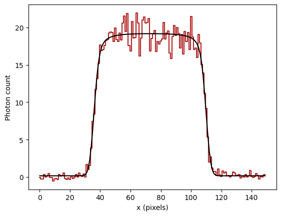
Plot data (red staircase curve – plasma fluorescence) and its expected value (black), evaluated with the initial parameter guess
plt.step(x, kymogram_no_rbc_mean/GAIN, where='mid', c='firebrick')
plt.plot(x, L_plasma_no_glx(x, *p0_B), c='k')

plt.xlabel('x (pixels)')
plt.ylabel('Photon count')
Text(0, 0.5, 'Photon count')
Fit model
opt_res_B = track_vessel.mle(x,
                             kymogram_no_rbc_mean,
                             L_plasma_no_glx,
                             p0_B,
                             N_AVER,
                             ALPHA,
                             SIGMA,
                             minimize_options=dict(gtol=1e-3))
opt_res_B
  message: Optimization terminated successfully.
  success: True
   status: 0
      fun: 575.8926283948229
        x: [ 7.290e+01  2.367e+00  7.748e+00  3.770e+01  1.931e+01
             1.691e-01]
      nit: 10
      jac: [ 5.341e-05  9.918e-05  3.815e-05  1.526e-05 -9.155e-05
             3.052e-05]
 hess_inv: [[ 2.462e-03  5.004e-04 ... -3.205e-04 -2.974e-05]
            [ 5.004e-04  1.285e-02 ... -8.603e-03 -8.372e-04]
            ...
            [-3.205e-04 -8.603e-03 ...  2.221e-02  4.151e-04]
            [-2.974e-05 -8.372e-04 ...  4.151e-04  9.986e-04]]
     nfev: 112
     njev: 16
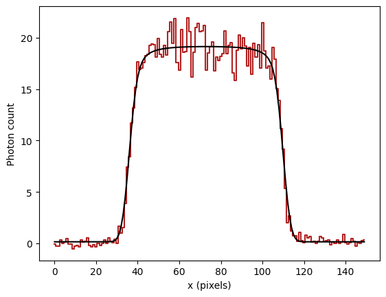
Plot data (red staircase curves – plasma fluorescence) and its fitted expected value (black)
plt.step(x, kymogram_no_rbc_mean/GAIN, where='mid', c='firebrick')
plt.plot(x, L_plasma_no_glx(x, *opt_res_B.x), c='k')

plt.xlabel('x (pixels)')
plt.ylabel('Photon count')
Text(0, 0.5, 'Photon count')
List fitted parameters and their error bars
p_calib = misc.fitted_params(opt_res_B, ['xc', 's_xy', 'l', 'R_lum', 'I', 'b'])
p_calib
{'xc': (72.90419879479425, 0.04961716371214573),
 's_xy': (2.3667182148769137, 0.11337571432485805),
 'l': (7.7483886098670025, 0.7333722183491217),
 'R_lum': (37.69942611694723, 0.1302062414720259),
 'I': (19.30678334496567, 0.1490378244767953),
 'b': (0.16913187094047408, 0.031601330942727275)}
Preparing fluorescence line-profiles for fitting#
Block-average kymogram (10 line-scans per block) to reduce noise, yielding line-profiles of fluorescence
n_block = 10

kymogram_blocked = kymogram[:-(kymogram.shape[0]%n_block), :].reshape((kymogram.shape[0]//n_block, n_block, nx))
kymogram_blocked_mean = kymogram_blocked.mean(axis=1)
Plot block-averaged kymogram
fig, ax = plt.subplots(figsize=(18, 3))

ax.imshow(kymogram_blocked_mean.T,
           cmap='afmhot',
           vmin=kymogram_blocked_mean.min(),
           vmax=kymogram_blocked_mean.max(),
           aspect=0.3,
           interpolation='none'
         )

ax.set_xlabel('Time (pix)')
ax.set_ylabel('x (pix)')
Text(0, 0.5, 'x (pix)')
Removing parts of the fluorescence profiles affected by RBCs. We can use estimated center position and capillary radius from the calibration to calculate positions of the edges of the plasma cylinder
edge1, edge2 = opt_res_B.x[0] - opt_res_B.x[3], opt_res_B.x[0] + opt_res_B.x[3]
fig, ax = plt.subplots(figsize=(18, 3))

ax.imshow(kymogram_blocked_mean.T,
           cmap='afmhot',
           vmin=kymogram_blocked_mean.min(),
           vmax=kymogram_blocked_mean.max(),
           aspect=0.3,
         )

ax.axhline(y=edge1, ls='--', color='w')
ax.axhline(y=edge2, ls='--', color='w')

ax.set_xlabel('Time (pix)')
ax.set_ylabel('x (pix)')
Text(0, 0.5, 'x (pix)')
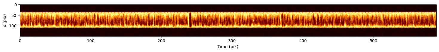
We want to extract fluorescence only near the edges of the capillary, where the fluorescence is not affected by RBCs
x_index_edge1, x_index_edge2 = np.searchsorted(x, [edge1, edge2])
x_edge1 = x[:x_index_edge1]
y_edge1 = kymogram_blocked_mean[:, :x_index_edge1]

x_edge2 = x[x_index_edge2:]
y_edge2 = kymogram_blocked_mean[:, x_index_edge2:]
Show extracted tails of fluorescence at three time points (beginning, middle, ending)
fig, ax = plt.subplots(figsize=(8, 4))

ax.set_xlabel('x (pixel)')
ax.set_ylabel('Photon count')

ax.step(x, kymogram_no_rbc_mean/GAIN, where='mid', c='k', lw=1)

t_indexes = [0, 300, -1]
colors = ['navy', 'r', 'c']

for ti, ci in zip(t_indexes, colors):
    ax.step(x_edge1, y_edge1[ti]/GAIN, where='mid', c=ci)
    ax.step(x_edge2, y_edge2[ti]/GAIN, where='mid', c=ci)
Tracking the capillary’s center and radius by fitting line-profiles of fluorescence#
Function describing the fluoresence intensity on the line profiles, L_plasma_no_glx, has six parameters: \(x_c\), \(\sigma_{xy}\), \(\lambda\), \(R_{lum}\), \(I\), \(b\). We set \(\sigma_{xy}\), \(\lambda\), \(I\), and \(b\) to the values obtained from the calibration and only fit \(x_c\) and \(R_{lum}\) for each line-profile of fluorescence. This new function, depending only on \(x_c\) and \(R_{lum}\), is denoted L_fit below.
fixed_args = {name: p_calib[name][0] for name in ['s_xy', 'l', 'I', 'b']}

L_fit = lambda x, xc, R_lum: L_plasma_no_glx(x, xc, p_calib['s_xy'][0], p_calib['l'][0], R_lum, p_calib['I'][0], p_calib['b'][0])
Concatenate the line-profiles
x_no_rbc = np.hstack([x_edge1, x_edge2])
y_no_rbc = np.hstack([y_edge1, y_edge2])
Fit all line-profiles
result = [] # contains fitted parameters for each line-profile

for i, y_i in enumerate(y_no_rbc, start=1):

    opt_res_i = track_vessel.mle(x_no_rbc,
                                 y_i,
                                 L_fit,
                                 [p_calib['xc'][0], p_calib['R_lum'][0]], # initial guess from the calibration parameters
                                 n_block,
                                 ALPHA,
                                 SIGMA,
                                 minimize_options=dict(gtol=1e-3))

    result.append(misc.fitted_params(opt_res_i, ['xc', 'R_lum']))

    if i%50 == 0:
        print(f'{i}/{y_no_rbc.shape[0]} fits completed')
50/589 fits completed
100/589 fits completed
150/589 fits completed
200/589 fits completed
250/589 fits completed
300/589 fits completed
350/589 fits completed
400/589 fits completed
450/589 fits completed
500/589 fits completed
550/589 fits completed
/home/docs/checkouts/readthedocs.org/user_builds/sl2pm/envs/latest/lib/python3.11/site-packages/sl2pm/models.py:80: RuntimeWarning: invalid value encountered in sqrt
  integrand = gaussian(R - X_PSF, s_xy)*(1 - np.exp(-np.sqrt(R_lum**2 - R**2)/l))
Visualizing the tracking results#
R_lum_fit = np.array([fit_i['R_lum'] for fit_i in result])
xc_fit = np.array([fit_i['xc'] for fit_i in result])
Calculate recording times for the block-averaged profiles in seconds (the raw kymogram, plasma_kymogram_long.npy, is 10 sec long)
t = np.linspace(0, 10, y_no_rbc.shape[0]) #
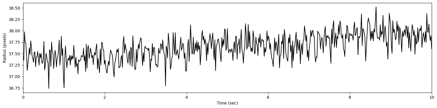
Plot capillary radius as a function of time
fig, ax = plt.subplots(figsize=(18, 4))
ax.set_xlabel('Time (sec)')
ax.set_ylabel('Radius (pixels)')

ax.plot(t, R_lum_fit[:, 0], ls='-', marker='', c='k')
ax.set_xlim(t[0], t[-1])
(0.0, 10.0)
Plot center positions as a function of time
fig, ax = plt.subplots(figsize=(18, 4))
ax.set_xlabel('Time (sec)')
ax.set_ylabel('Center position (pixels)')

ax.plot(t, xc_fit[:, 0], ls='-', marker='', c='k')
ax.set_xlim(t[0], t[-1])
(0.0, 10.0)
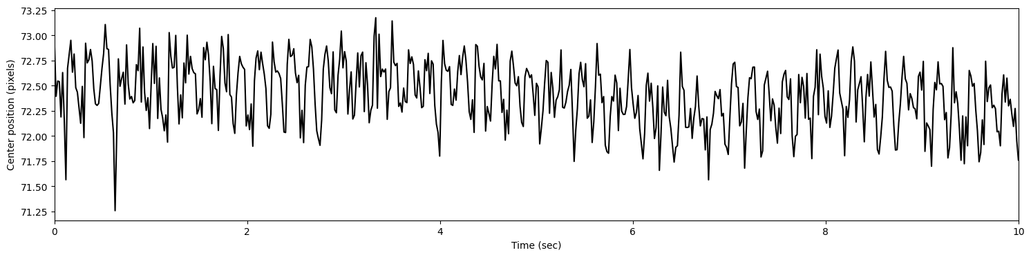
Note the heartbeats (~5-6 Hz) visible in both the radius and center position traces
Inspecting the fits#
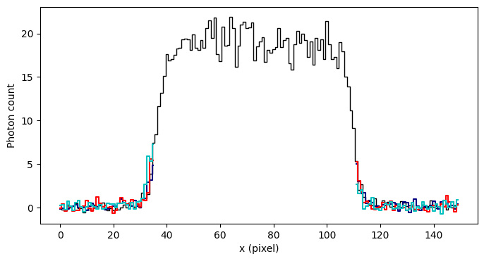
We selected four fitted profiles and plotted them below
red curves: Two parts of the fluorescence profile not affected by RBCs. We fit these data.
blue curve: Full fluorescence profile, including the central part affected by RBCs
black curve: Fits of the red curves with L_plasma_no_glx (with fixed parameters from the calibration, see above)
indexes_to_check = np.arange(0, kymogram_blocked_mean.shape[0], 100)

for i in indexes_to_check:

    fig, ax = plt.subplots()

    ax.set_xlabel('x (pixel)')
    ax.set_ylabel('Photon count')

    ax.step(x_edge1, y_edge1[i]/GAIN, c='r', where='mid')
    ax.step(x_edge2, y_edge2[i]/GAIN, c='r', where='mid')
    ax.step(x, kymogram_blocked_mean[i]/GAIN, c='royalblue', lw=0.5, where='mid')

    y_fit_i = L_fit(x, result[i]['xc'][0], result[i]['R_lum'][0])
    ax.plot(x, y_fit_i, c='k')
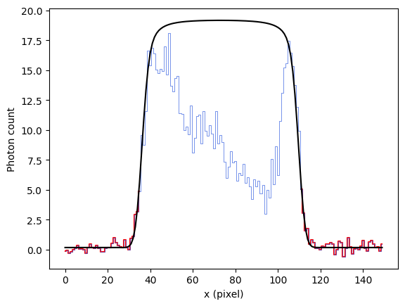
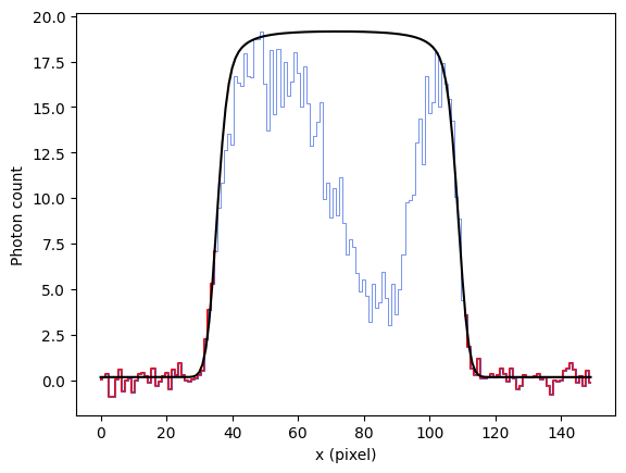
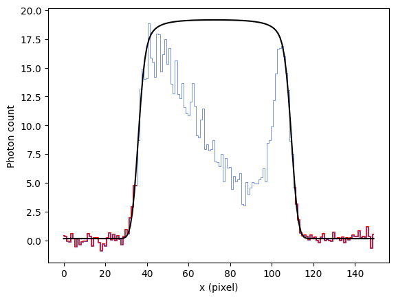
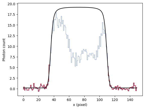
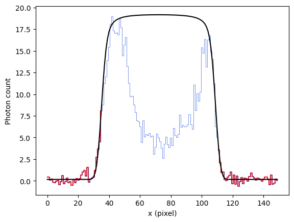
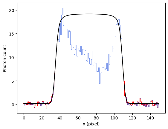
The fits show consistency with the data, i.e., the black fitted curve goes through the red curves. When this is the case, you can trust the estimates of the radius and capillary center position.