Demo for how to track a blood vessel in time and calibrate the microscope’s PSF in a single fit (“ultimate fit”).#
import matplotlib.pyplot as plt
import numpy as np

from sl2pm import track_vessel
from sl2pm.models import L_multi, L_multi_plasma, L_multi_wall
from sl2pm import misc
Protocol A: The Ultimate Fit (both plasma and wall fluorescence)#
Load wall- and plasma kymograms and average line-scans over time
kymo_wall = np.load('wall.npy')
kymo_plasma = np.load('plasma.npy')

nt, nx = kymo_wall.shape
x = np.arange(nx)

kymo_wall = kymo_wall.reshape((2, nt//2, nx)).mean(axis=1)
kymo_plasma = kymo_plasma.reshape((2, nt//2, nx)).mean(axis=1)

N_AVER = nt//2
Enter PMT parameters (known from the calibration)
ALPHA = 0.452
SIGMA = 6.0
GAIN = 3/ALPHA
Make an initial parameter guess
xc, s_xy, l, R_lum, R_wall, s_gcx, a1, Iw, Ip, b_plasma, b_tissue_wall, b_tissue_plasma = track_vessel.ols_wall_plasma(kymo_wall[0]/GAIN,
                                    kymo_plasma[0]/GAIN,
                                    sigma_blur=1.5)

p0_A = [s_xy, l, R_wall - R_lum, s_gcx, b_plasma, b_tissue_wall, b_tissue_plasma,
        *(2*[Iw]), *(2*[Ip]), *(2*[R_wall]), *(2*[xc]), *(2*[a1])]
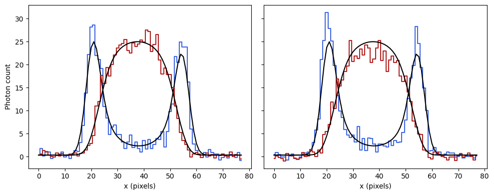
Plot data (staircase curves; blue – wall fluorescence, red – plasma fluorescence) and its expected value (black), evaluated with the initial parameter guess
[[w1_A0, p1_A0], [w2_A0, p2_A0]] = L_multi(x, *p0_A)

fig, [ax1, ax2] = plt.subplots(1, 2, sharey=True, figsize=(10, 4))

# First time point
ax1.step(x, kymo_wall[0]/GAIN, where='mid', c='royalblue')
ax1.plot(x, w1_A0, c='k')

ax1.step(x, kymo_plasma[0]/GAIN, where='mid', c='firebrick')
ax1.plot(x, p1_A0, c='k')

# Second time point
ax2.step(x, kymo_wall[1]/GAIN, where='mid', c='royalblue')
ax2.plot(x, w2_A0, c='k')

ax2.step(x, kymo_plasma[1]/GAIN, where='mid', c='firebrick')
ax2.plot(x, p2_A0, c='k')

ax1.set_xlabel('x (pixels)')
ax2.set_xlabel('x (pixels)')
ax1.set_ylabel('Photon count')

plt.tight_layout()
Fit the model
opt_res_A = track_vessel.mle(x,
                             np.array([*zip(kymo_wall, kymo_plasma)]),
                             L_multi,
                             p0_A,
                             N_AVER,
                             ALPHA,
                             SIGMA,
                             minimize_options=dict(gtol=1e-3))
opt_res_A
  message: Optimization terminated successfully.
  success: True
   status: 0
      fun: 1148.3533813410195
        x: [ 2.107e+00  8.063e+00 ... -6.067e-02 -1.073e-01]
      nit: 41
      jac: [ 5.341e-04 -6.104e-04 ...  9.155e-05 -4.883e-04]
 hess_inv: [[ 1.912e-03 -3.659e-02 ...  1.812e-05  2.363e-06]
            [-3.659e-02  1.355e+00 ... -6.204e-04  1.545e-04]
            ...
            [ 1.812e-05 -6.204e-04 ...  1.437e-04  6.624e-07]
            [ 2.363e-06  1.545e-04 ...  6.624e-07  1.439e-04]]
     nfev: 864
     njev: 48
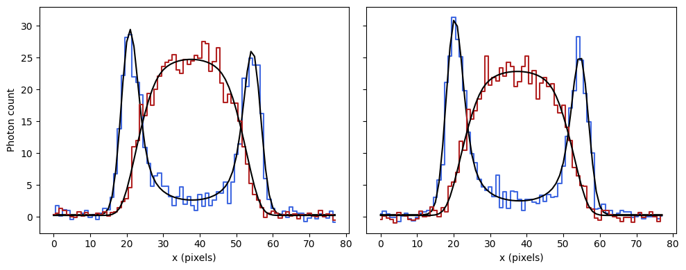
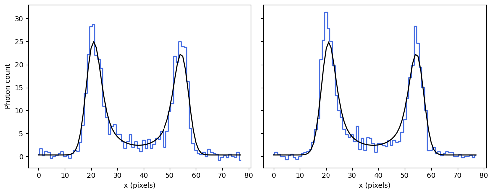
Plot data (staircase curves; blue – wall fluorescence, red – plasma fluorescence) and its fitted expected value (black)
[[w1_A, p1_A], [w2_A, p2_A]] = L_multi(x, *opt_res_A.x)

fig, [ax1, ax2] = plt.subplots(1, 2, sharey=True, figsize=(10, 4))

# First time point
ax1.step(x, kymo_wall[0]/GAIN, where='mid', c='royalblue')
ax1.plot(x, w1_A, c='k')

ax1.step(x, kymo_plasma[0]/GAIN, where='mid', c='firebrick')
ax1.plot(x, p1_A, c='k')

# Second time point
ax2.step(x, kymo_wall[1]/GAIN, where='mid', c='royalblue')
ax2.plot(x, w2_A, c='k')

ax2.step(x, kymo_plasma[1]/GAIN, where='mid', c='firebrick')
ax2.plot(x, p2_A, c='k')

ax1.set_xlabel('x (pixels)')
ax2.set_xlabel('x (pixels)')
ax1.set_ylabel('Photon count')

plt.tight_layout()
List fitted parameters and their error bars
misc.fitted_params(opt_res_A, ['s_xy', 'l', 'dR', 's_gcx', 'b_plasma', 'b_tissue_wall', 'b_tissue_plasma', 'Iw1', 'Iw2', 'Ip1', 'Ip2', 'R_w1', 'R_w2', 'xc1', 'xc2', 'a1_1', 'a1_2'])
{'s_xy': (2.1071911141312105, 0.04373039040974113),
 'l': (8.063225182533367, 1.1641381033674696),
 'dR': (6.12082225946461, 0.6617343691975737),
 's_gcx': (6.94706197085172, 1.2868966705804914),
 'b_plasma': (-0.3290971754974562, 0.8386670358311792),
 'b_tissue_wall': (0.3355322460483374, 0.05325942967396143),
 'b_tissue_plasma': (0.2328174967195196, 0.04761337236719887),
 'Iw1': (201.88541470253577, 13.036613386300983),
 'Iw2': (203.46261190331586, 13.225417754842288),
 'Ip1': (29.20484437073755, 1.3560317322505135),
 'Ip2': (26.72968847740829, 1.2306034735747484),
 'R_w1': (17.559087551754963, 0.07906942465323095),
 'R_w2': (17.948498267455264, 0.07777311245674709),
 'xc1': (37.61732210193796, 0.034138084841778625),
 'xc2': (37.42960653780086, 0.03474461823660636),
 'a1_1': (-0.06067336129407629, 0.011985716687867848),
 'a1_2': (-0.10730088541341448, 0.011995593295493497)}
Protocol B: The Ultimate Fit (only plasma fluorescence)#
Load plasma kymograms and average line-scans over time
kymo_plasma = np.load('plasma.npy')

nt, nx = kymo_plasma.shape
x = np.arange(nx)

kymo_plasma = kymo_plasma.reshape((2, nt//2, nx)).mean(axis=1)

N_AVER = nt//2
Enter PMT parameters (known from the calibration)
ALPHA = 0.452
SIGMA = 6.0
GAIN = 3/ALPHA
Make an initial parameter guess
xc, s_xy, l, R_lum, I, b = track_vessel.ols_plasma(kymo_plasma[0]/GAIN, sigma_blur=1.5)

p0_B = [s_xy, l, b, *(2*[I]), *(2*[R_lum]), *(2*[xc])]
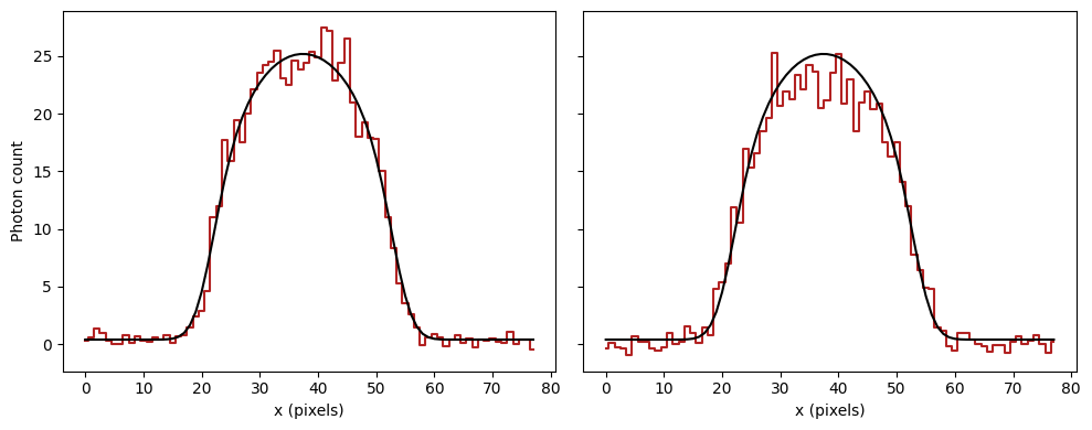
Plot data (red staircase curve – plasma fluorescence) and its expected value (black), evaluated with the initial parameter guess
p1_B0, p2_B0 = L_multi_plasma(x, *p0_B)

fig, [ax1, ax2] = plt.subplots(1, 2, sharey=True, figsize=(10, 4))

# First time point
ax1.step(x, kymo_plasma[0]/GAIN, where='mid', c='firebrick')
ax1.plot(x, p1_B0, c='k')

# Second time point
ax2.step(x, kymo_plasma[1]/GAIN, where='mid', c='firebrick')
ax2.plot(x, p2_B0, c='k')

ax1.set_xlabel('x (pixels)')
ax2.set_xlabel('x (pixels)')
ax1.set_ylabel('Photon count')

plt.tight_layout()
Fit the model
opt_res_B = track_vessel.mle(x,
                             kymo_plasma,
                             L_multi_plasma,
                             p0_B,
                             N_AVER,
                             ALPHA,
                             SIGMA,
                             minimize_options=dict(gtol=1e-3))
opt_res_B
  message: Optimization terminated successfully.
  success: True
   status: 0
      fun: 525.965011547179
        x: [-2.438e+00  3.010e+01  2.375e-01  6.033e+01  5.259e+01
             1.641e+01  1.725e+01  3.740e+01  3.732e+01]
      nit: 45
      jac: [-6.104e-05  8.392e-05 -3.052e-04 -7.629e-05  1.526e-05
            -6.332e-04 -2.289e-05  7.629e-06  1.297e-04]
 hess_inv: [[ 2.694e-02  1.757e+00 ...  6.142e-04  2.977e-04]
            [ 1.757e+00  2.187e+02 ...  5.600e-02  3.203e-02]
            ...
            [ 6.142e-04  5.600e-02 ...  5.970e-03 -4.483e-06]
            [ 2.977e-04  3.203e-02 ... -4.483e-06  6.354e-03]]
     nfev: 600
     njev: 60
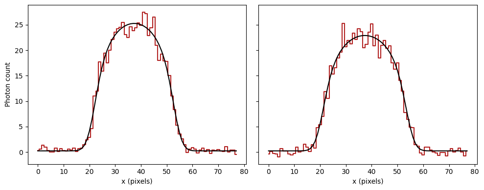
Plot data (red staircase curves – plasma fluorescence) and its fitted expected value (black)
p1_B, p2_B = L_multi_plasma(x, *opt_res_B.x)

fig, [ax1, ax2] = plt.subplots(1, 2, sharey=True, figsize=(10, 4))

# First time point
ax1.step(x, kymo_plasma[0]/GAIN, where='mid', c='firebrick')
ax1.plot(x, p1_B, c='k')

# Second time point
ax2.step(x, kymo_plasma[1]/GAIN, where='mid', c='firebrick')
ax2.plot(x, p2_B, c='k')

ax1.set_xlabel('x (pixels)')
ax2.set_xlabel('x (pixels)')
ax1.set_ylabel('Photon count')

plt.tight_layout()
List fitted parameters and their error bars
misc.fitted_params(opt_res_B, ['s_xy', 'l', 'b', 'I1', 'I2', 'R1', 'R2', 'xc1', 'xc2'])
{'s_xy': (-2.438335437280602, 0.16414329536021025),
 'l': (30.09840625987249, 14.787577271754804),
 'b': (0.23745278134530595, 0.05045385131679118),
 'I1': (60.32950595094914, 21.96619751700218),
 'I2': (52.58957900488604, 18.826035399510822),
 'R1': (16.407968319674183, 0.22339621144433755),
 'R2': (17.247534729965096, 0.24580537084363965),
 'xc1': (37.39772147466368, 0.07726415337169366),
 'xc2': (37.31662740028516, 0.07971198309695891)}
Protocol C: The Ultimate Fit (only wall fluorescence)#
Load wall kymograms and average line-scans over time
kymo_wall = np.load('wall.npy')

nt, nx = kymo_wall.shape
x = np.arange(nx)

kymo_wall = kymo_wall.reshape((2, nt//2, nx)).mean(axis=1)

N_AVER = nt//2
Enter PMT parameters (known from the calibration)
ALPHA = 0.452
SIGMA = 6.0
GAIN = 3/ALPHA
Make an initial parameter guess
xc, s_xy, l, R_wall, a1, I, b_plasma, b_tissue = track_vessel.ols_wall(kymo_wall[0]/GAIN, sigma_blur=1.5)

p0_C = [s_xy, l, b_plasma, b_tissue,
        *(2*[I]), *(2*[R_wall]), *(2*[xc]), *(2*[a1])]
Plot data (blue staircase curves – wall fluorescence) and its expected value (black), evaluated with the initial parameter guess
w1_C0, w2_C0 = L_multi_wall(x, *p0_C)

fig, [ax1, ax2] = plt.subplots(1, 2, sharey=True, figsize=(10, 4))

# First time point
ax1.step(x, kymo_wall[0]/GAIN, where='mid', c='royalblue')
ax1.plot(x, w1_C0, c='k')

# Second time point
ax2.step(x, kymo_wall[1]/GAIN, where='mid', c='royalblue')
ax2.plot(x, w2_C0, c='k')

ax1.set_xlabel('x (pixels)')
ax2.set_xlabel('x (pixels)')
ax1.set_ylabel('Photon count')

plt.tight_layout()
Fit the model
opt_res_C = track_vessel.mle(x,
                             kymo_wall,
                             L_multi_wall,
                             p0_C,
                             N_AVER,
                             ALPHA,
                             SIGMA,
                             minimize_options=dict(gtol=1e-3))
opt_res_C
  message: Optimization terminated successfully.
  success: True
   status: 0
      fun: 607.7487019395948
        x: [ 2.114e+00  7.833e+00 -1.582e-01  3.334e-01  1.993e+02
             2.008e+02  1.758e+01  1.791e+01  3.767e+01  3.745e+01
            -6.182e-02 -1.078e-01]
      nit: 33
      jac: [-6.866e-05  2.289e-05  3.052e-05  7.629e-06  0.000e+00
             0.000e+00  4.578e-05 -7.629e-06  2.289e-05 -3.052e-05
             6.866e-05  6.638e-04]
 hess_inv: [[ 1.779e-03 -2.964e-02 ...  1.342e-05  1.555e-05]
            [-2.964e-02  9.594e-01 ... -3.148e-04  1.086e-04]
            ...
            [ 1.342e-05 -3.148e-04 ...  1.490e-04  2.993e-06]
            [ 1.555e-05  1.086e-04 ...  2.993e-06  1.589e-04]]
     nfev: 533
     njev: 41
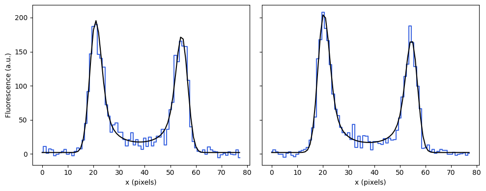
Plot data (blue staircase curves – wall fluorescence) and its fitted expected value (black)
w1_C, w2_C = L_multi_wall(x, *opt_res_C.x)

fig, [ax1, ax2] = plt.subplots(1, 2, sharey=True, figsize=(10, 4))

# First time point
ax1.step(x, kymo_wall[0], where='mid', c='royalblue')
ax1.plot(x, w1_C*GAIN, c='k')

# Second time point
ax2.step(x, kymo_wall[1], where='mid', c='royalblue')
ax2.plot(x, w2_C*GAIN, c='k')

ax1.set_xlabel('x (pixels)')
ax2.set_xlabel('x (pixels)')
ax1.set_ylabel('Fluorescence (a.u.)')

plt.tight_layout()
List fitted parameters and their error bars
misc.fitted_params(opt_res_C, ['s_xy', 'l', 'b_plasma', 'b_tissue', 'Iw1', 'Iw2', 'R_w1', 'R_w2', 'xc1', 'xc2', 'a1_1', 'a1_2'])
{'s_xy': (2.1141527067607195, 0.04217600526507939),
 'l': (7.832910936065337, 0.9794669972339229),
 'b_plasma': (-0.1581661959907053, 0.7092500981499678),
 'b_tissue': (0.33343901152764827, 0.053212776891061284),
 'Iw1': (199.32032625788366, 10.856472915494134),
 'Iw2': (200.84962419995642, 10.90825701009266),
 'R_w1': (17.582949773013944, 0.07318603612265313),
 'R_w2': (17.909231125925654, 0.07228926656488537),
 'xc1': (37.6706625521205, 0.03890618872099604),
 'xc2': (37.45022552487506, 0.03886071174925817),
 'a1_1': (-0.061818683251947476, 0.012205982956591902),
 'a1_2': (-0.10781024570651082, 0.012605991009184499)}